API reference guide#
LossModel#
Risk costing#
GEMAct costing model is based on the collective risk theory. The aggregate loss \(X\), also referred to as aggregate claim cost, is
where the following assumptions hold:
\(N\) is a random variable taking values in \(\mathbb{N}_0\) representing the claim frequency.
\(\left\{ Z_i\right\}_{i \in \mathbb{N}}\) is a sequence of i.i.d non-negative random variables independent of \(N\); \(Z\) is the random variable representing the individual (claim) loss.
Equation (1) is often referred to as the frequency-severity loss model representation. This can encompass common coverage modifiers present in (re)insurance contracts. More specifically, we consider:
For \(a \in [0, 1]\), the function \(Q_a\) apportioning the aggregate loss amount:
\[Q_a (X)= a X.\]
For \(c,d \geq 0\), the function \(L_{c, d}\) applied to the individual claim loss:
(2)#\[L_{c, d} (Z_i) = \min \left\{\max \left\{0, Z_i-d\right\}, c\right\}. %, \qquad c,d \geq 0.\]Herein, for each and every loss, the excess to a deductible \(d\) (sometimes referred to as priority) is considered up to a cover or limit \(c\). Similarly to the individual loss \(Z_i\), Formula (2) can be applied to the aggregate loss \(X\).
The expected value of the aggregate loss constitutes the building block of an insurance tariff. Listed below are some examples of basic reinsurance contracts whose pure premium can be computed with GEMAct.
The Quota Share (QS), where a share \(a\) of the aggregate loss ceded to the reinsurance (along with the respective premium) and the remaining part is retained:
\[\text{P}^{QS} = \mathbb{E}\left[ Q_a \left( X \right)\right].\]
The Excess-of-loss (XL), where the insurer cedes to the reinsurer each and every loss exceeding a deductible \(d\), up to an agreed limit or cover \(c\), with \(c,d \geq 0\):
\[\text{P}^{XL} = \mathbb{E}\left[ \sum_{i=1}^{N} L_{c,d} (Z_i) \right].\]
The Stop Loss (SL), where the reinsurer covers the aggregate loss exceedance of a (aggregate) deductible \(v\), up to a (aggregate) limit or cover \(u\), with \(u,v \geq 0\):
\[\text{P}^{SL} = \mathbb{E}\left[ L_{u, v} (X) \right].\]
The Excess-of-loss with reinstatements (RS) (Sundt [Sun91]). Assuming the aggregate cover \(u\) is equal to \((K + 1) c `, with :math:`K \in \mathbb{Z}^+\):
(3)#\[\text{P}^{RS} = \frac{\mathbb{E}\left[ L_{u, v} (X) \right]}{1+\frac{1}{c} \sum_{k=1}^K l_k \mathbb{E}\left[ L_{c, (k-1)c+v}(X) \right]}.\]Where \(K\) is the number of reinstatement layers and \(l_k \in [0, 1]\) is the reinstatement premium percentage, with \(k=1, \ldots, K\). When \(l_k = 0\), the \(k\)-th resinstatement is said to be free.
The following table gives the correspondence between the LossModel class attributes and our costing model as presented below.
Costing model notation |
Parametrization in |
|---|---|
\(d\) |
deductible |
\(c\) |
cover |
\(v\) |
aggr_deductible |
\(u\) |
aggr_cover |
\(K\) |
n_reinst |
\(c_{k}\) |
reinst_percentage |
\(\alpha\) |
share |
For additional information the reader can refer to Klugman and Panjer [KP19], Sundt [Sun91]. Further details on the computational methods to approximate the aggregate loss distribution can be found in Klugman and Panjer [KP19], and Embrechts and Frei [EF08].
Example#
Below is an example of costing an XL contract with reinstatements:
from gemact.lossmodel import Frequency, Severity, PolicyStructure, LossModel
lossmodel_RS = LossModel(
 frequency=Frequency(
     dist='poisson',
     par={'mu': 1.5}
 ),
 severity=Severity(
     par= {'loc': 0,
           'scale': 83.34,
           'c': 0.834},
     dist='genpareto'
 ),
 policystructure=PolicyStructure(
     layers=Layer(
         cover=100,
         deductible=0,
         aggr_deductible=100,
         reinst_share=0.5,
         n_reinst=2
     )
 ),
 aggr_loss_dist_method='fft',
 sev_discr_method='massdispersal',
 n_aggr_dist_nodes=int(100000)
 )
 lossmodel_RS.print_costing_specs()
Severity discretization#
When passing from a continuous distribution to an arithmetic distribution, it is important to preserve the distribution properties, either locally or globally. Given a bandiwith (or discretization step) \(h\) and a number of nodes \(M\), in Klugman and Panjer [KP19] the method of mass dispersal and the method of local moments matching work as follows.
Method of mass dispersal
Method of local moments matching
The following approach is applied to preserve the global mean of the distribution.
In addition to these two methods, our package also provides the methods of upper and lower discretizations.
Example#
An example of code to implement severity discretization is given below:
from gemact.lossmodel import Severity
import numpy as np

severity=Severity(
    par= {'loc': 0, 'scale': 83.34, 'c': 0.834},
    dist='genpareto'
)

massdispersal = severity.discretize(
discr_method='massdispersal',
n_discr_nodes=50000,
discr_step=.01,
deductible=0
)

localmoments = severity.discretize(
discr_method='localmoments',
n_discr_nodes=50000,
discr_step=.01,
deductible=0
)

meanMD = np.sum(massdispersal['sev_nodes'] * massdispersal['fj'])
meanLM = np.sum(localmoments['sev_nodes'] * localmoments['fj'])

print('Original mean: ', severity.model.mean())
print('Mean (mass dispersal): ', meanMD)
print('Mean (local moments): ', meanLM)
LossReserve#
Claims reserving#
GEMAct provides a software implementation of average cost methods for claims reserving based on the collective risk model framework.
The methods implemented are the Fisher-Lange in Fisher et al. [FLB99] the collective risk model for claims reserving in Ricotta and Clemente [RC16].
It allows for tail estimates and assumes the triangular inputs to be provided as a numpy.ndarray with two equal dimensions (I,J), where I=J.
The aim of average cost methods is to model incremental payments as in equation (11).
where \(n_{i,j}\) is the number of payments in the cell \(i,j\) and \(m_{i,j}\) is the average cost in the cell \(i,j\).
Example#
It is possible to use the module gemdata to test GEMAct average cost methods:
from gemact import gemdata
ip_ = gemdata.incremental_payments
in_ = gemdata.incurred_number
cp_ = gemdata.cased_payments
cn_= gemdata.cased_number
reported_ = gemdata.reported_claims
claims_inflation = gemdata.claims_inflation
An example of Fisher-Lange implementation:
from gemact.lossreserve import AggregateData, ReservingModel
from gemact import gemdata

ip_ = gemdata.incremental_payments
in_ = gemdata.incurred_number
cp_ = gemdata.cased_payments
cn_= gemdata.cased_number
reported_ = gemdata.reported_claims
claims_inflation = gemdata.claims_inflation

ad = AggregateData(
  incremental_payments=ip_,
  cased_payments=cp_,
  cased_number=cn_,
  reported_claims=reported_,
  incurred_number=in_
  )

rm = ReservingModel(
  tail=True,
  reserving_method="fisher_lange",
  claims_inflation=claims_inflation
  )

lm = gemact.LossReserve(
  data=ad,
  reservingmodel=rm
  )
Observe the CRM for reserving requires different model assumptions:
from gemact import gemdata

ip_ = gemdata.incremental_payments
in_ = gemdata.incurred_number
cp_ = gemdata.cased_payments
cn_= gemdata.cased_number
reported_ = gemdata.reported_claims
claims_inflation = gemdata.claims_inflation

from gemact.lossreserve import AggregateData, ReservingModel, LossReserve
ad = AggregateData(
    incremental_payments=ip_,
    cased_payments=cp_,
    cased_number=cn_,
    reported_claims=reported_,
    incurred_number=in_)


mixing_fq_par = {'a': 1 / .08 ** 2,  # mix frequency
                     'scale': .08 ** 2}

mixing_sev_par = {'a': 1 / .08 ** 2, 'scale': .08 ** 2}  # mix severity
czj = gemdata.czj
claims_inflation= gemdata.claims_inflation

rm =  ReservingModel(tail=True,
         reserving_method="crm",
         claims_inflation=claims_inflation,
         mixing_fq_par=mixing_fq_par,
         mixing_sev_par=mixing_sev_par,
         czj=czj)

#Loss reserving: instance lr
lm = LossReserve(data=ad,
                 reservingmodel=rm)
LossAggregation#
Loss aggregation#
The probability in equation (12) can be approximated iteratively via the AEP algorithm, which is implemented for the first time in the GEMAct package, under the following assumptions:
Assuming:
\(𝑋=(X_i, \ldots, X_d)\) vector of strictly positive random components.
The joint c.d.f. \(H(x_1,…,x_d )=P\left[ X_1 +\ldots +X_d \right]\) is known or it can be computed numerically.
Refer to Arbenz et al. [AEP11] for an extensive explanation on the AEP algorithm. It is possible to use a MC simulation for comparison.
Example#
Example code under a clayton assumption:
from gemact.lossaggregation import LossAggregation, Copula, Margins

lossaggregation = LossAggregation(
margins=Margins(
dist=['genpareto', 'lognormal'],
par=[{'loc': 0, 'scale': 1/.9, 'c': 1/.9}, {'loc': 0, 'scale': 10, 'shape': 1.5}],
),
copula=Copula(
dist='frank',
par={'par': 1.2, 'dim': 2}
),
n_sim=500000,
random_state=10,
n_iter=8
)
s = 300 # arbitrary value
p_aep = lossaggregation.cdf(x=s, method='aep')
print('P(X1+X2 <= s) = ', p_aep)
p_mc = lossaggregation.cdf(x=s, method='mc')
print('P(X1+X2 <= s) = ', p_mc)
The distributions module#
Poisson#
Parametrization#
For a more detailed explanation refer to SciPy Poisson distribution documentation, see Virtanen et al. [VGO+20].
Given \(\mu \geq 0\) and \(k \geq 0\).
Example code on the usage of the Poisson class:
from gemact import distributions
import numpy as np
mu = 4
dist = distributions.Poisson(mu=mu)
seq = np.arange(0,20)
nsim = int(1e+05)

# Compute the mean via pmf
mean = np.sum(dist.pmf(seq)*seq)
variance = np.sum(dist.pmf(seq)*(seq-mean)**2)

print('Mean',mean)
print('Theoretical mean', dist.mean())
print('Variance', variance)
print('Theoretical variance', dist.var())
#compare with simulations
print('Simulated mean', np.mean(dist.rvs(nsim)))
print('Simulated variance', np.var(dist.rvs(nsim)))
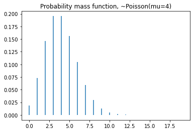
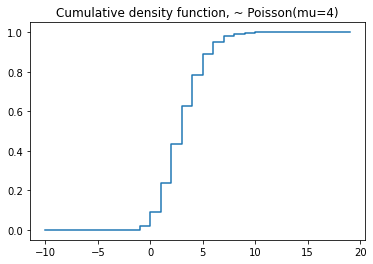
Then, use matplotlib library to show the pmf and the cdf of a Poisson:
import matplotlib.pyplot as plt

#pmf
plt.vlines(x=seq, ymin=0, ymax=dist.pmf(seq))
plt.title('Probability mass function, ~Poisson(mu=4)')

#cdf
plt.step(np.arange(-2,20), dist.cdf(np.arange(-2,20)),'-', where='pre')
plt.title('Cumulative distribution function, ~ Poisson(mu=4)')
Binom#
Parametrization#
For a more detailed explanation refer to SciPy Binomial distribution documentation, see Virtanen et al. [VGO+20].
for \(k \in\{0,1, \ldots, n\}, 0 \leq p \leq 1\)
Example code on the usage of the Binom class:
from gemact import distributions
import numpy as np

n = 10
p = 0.5
dist = distributions.Binom(n=n, p=p)
seq = np.arange(0,20)
nsim = int(1e+05)

# Compute the mean via pmf
mean=np.sum(dist.pmf(seq)*seq)
variance=np.sum(dist.pmf(seq)*(seq-mean)**2)

print('Mean',mean)
print('Theoretical mean',dist.mean())
print('Variance',variance)
print('Theoretical variance',dist.var())
#compare with simulations
print('Simulated mean',np.mean(dist.rvs(nsim)))
print('Simulated variance',np.var(dist.rvs(nsim)))
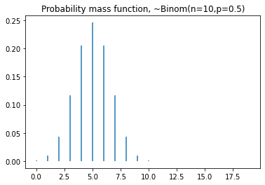
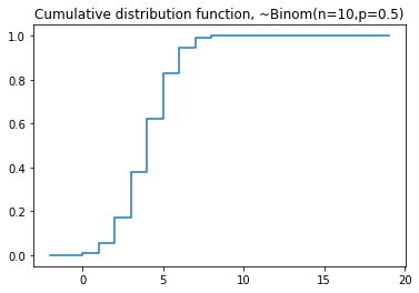
Then, use matplotlib library to show the pmf and the cdf of a Poisson:
import matplotlib.pyplot as plt
#pmf
plt.vlines(x=seq, ymin=0, ymax=dist.pmf(seq))
plt.title('Probability mass function, ~Binom(n=10,p=0.5)')

#cdf
plt.step(np.arange(-2,20),dist.cdf(np.arange(-2,20)),'-', where='pre')
plt.title('Cumulative distribution function, ~Binom(n=10,p=0.5)')
Geom#
Parametrization#
For a more detailed explanation refer to the SciPy Geometric distribution documentation, see Virtanen et al. [VGO+20]..
for \(k \geq 1,0<p \leq 1\)
Example code on the usage of the Geom class:
from gemact import distributions
import numpy as np

p=0.8
dist=distributions.Geom(p=p)
seq=np.arange(0,100,.001)
nsim=int(1e+05)

# Compute the mean via pmf
mean=np.sum(dist.pmf(seq)*seq)
variance=np.sum(dist.pmf(seq)*(seq-mean)**2)

print('Mean',mean)
print('Theoretical mean',dist.mean())
print('Variance',variance)
print('Theoretical variance',dist.var())
#compare with simulations
print('Simulated mean',np.mean(dist.rvs(nsim)))
print('Simulated variance',np.var(dist.rvs(nsim)))
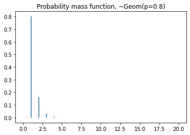
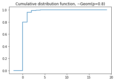
Then, use matplotlib library to show the pmf and the cdf of a Geom:
import matplotlib.pyplot as plt

#pmf
plt.vlines(x=seq, ymin=0, ymax=dist.pmf(seq))
plt.title('Probability mass function, ~Geom(p=0.8)')

#cdf
plt.step(np.arange(-2,20),dist.cdf(np.arange(-2,20)),'-', where='pre')
plt.title('Cumulative distribution function, ~Geom(p=0.8)')
NegBinom#
Parametrization#
For a more detailed explanation refer to the SciPy Negative Binomial documentation, see Virtanen et al. [VGO+20].
for \(k \geq 0,0<p \leq 1\)
Example code on the usage of the NegBinom class:
from gemact import distributions
import numpy as np

n = 10
p = .5
dist = distributions.NegBinom(n=n, p=p)
seq = np.arange(0,100,.001)
nsim = int(1e+05)

# Compute the mean via pmf
mean = np.sum(dist.pmf(seq)*seq)
variance = np.sum(dist.pmf(seq)*(seq-mean)**2)

print('Mean', mean)
print('Theoretical mean', dist.mean())
print('Variance', variance)
print('Theoretical variance', dist.var())
#compare with simulations
print('Simulated mean', np.mean(dist.rvs(nsim)))
print('Simulated variance', np.var(dist.rvs(nsim)))
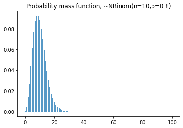
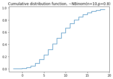
Then, use matplotlib library to show the pmf and the cdf of a NegBinom:
import matplotlib.pyplot as plt
#pmf
plt.vlines(x=seq, ymin=0, ymax=dist.pmf(seq))
plt.title('Probability mass function, ~NegBinom(n=10,p=0.8)')

#cdf
plt.step(np.arange(-2,20),dist.cdf(np.arange(-2,20)),'-', where='pre')
plt.title('Cumulative distribution function, ~NegBinom(n=10,p=0.8)')
Logser#
Parametrization#
For a more detailed explanation refer to the SciPy Logarithmic distribution documentation, see Virtanen et al. [VGO+20].
Given \(0 < p < 1\) and \(k \geq 1\).
Example code on the usage of the Logser class:
from gemact import distributions
import numpy as np

dist=distributions.Logser(p=.5)
seq=np.arange(0,30,.001)
nsim=int(1e+05)

# Compute the mean via pmf
mean=np.sum(dist.pmf(seq)*seq)
variance=np.sum(dist.pmf(seq)*(seq-mean)**2)

print('Mean',mean)
print('Variance',variance)
#compare with simulations
print('Simulated mean',np.mean(dist.rvs(nsim)))
print('Simulated variance',np.var(dist.rvs(nsim)))
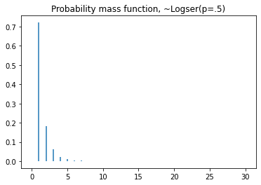
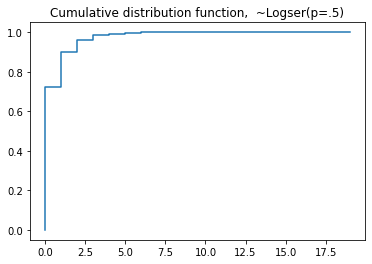
Then, use matplotlib library to show the pmf and the cdf of a Logser:
import matplotlib.pyplot as plt

#pmf
plt.vlines(x=seq, ymin=0, ymax=dist.pmf(seq))
plt.title('Probability mass function, ~Logser(p=.5)')

#cdf
plt.step(np.arange(0,20),dist.cdf(np.arange(0,20)),'-', where='pre')
plt.title('Cumulative distribution function,  ~Logser(p=.5)')
ZTPoisson#
Parametrization#
Let \(P(z)\) denote the probability generating function of a Poisson distribution.
\(p_{0}\) is \(p_{0}=P[z=0]\).
The probability generating function of a Zero-Truncated poisson is defined in equation (18).
Example code on the usage of the ZTPoisson class:
from gemact import distributions
import numpy as np

mu=2
dist=distributions.ZTpoisson(mu=mu)
seq=np.arange(0,30,.001)
nsim=int(1e+05)

# Compute the mean via pmf
mean=np.sum(dist.pmf(seq)*seq)
variance=np.sum(dist.pmf(seq)*(seq-mean)**2)

print('Mean',mean)
print('Variance',variance)
#compare with simulations
print('Simulated mean',np.mean(dist.rvs(nsim)))
print('Simulated variance',np.var(dist.rvs(nsim)))
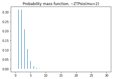
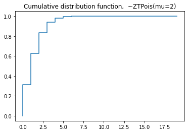
Then, use matplotlib library to show the pmf and the cdf of a ZTPoisson:
import matplotlib.pyplot as plt

#pmf
plt.vlines(x=seq, ymin=0, ymax=dist.pmf(seq))
plt.title('Probability mass function, ~ZTPoisson(mu=2)')
#cdf
plt.step(np.arange(0,20),dist.cdf(np.arange(0,20)),'-', where='pre')
plt.title('Cumulative distribution function,  ~ZTPoisson(mu=2)')
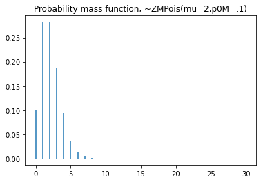
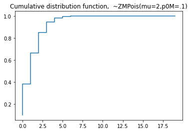
ZMPoisson#
Parametrization#
Let \(P(z)\) denote the probability generating function of a Poisson distribution.
\(p_{0}\) is \(p_{0}=P[z=0]\).
The probability generating function of a Zero-Truncated poisson is defined in equation (19)
Example code on the usage of the ZMPoisson class:
from gemact import distributions
import numpy as np

mu=2
p0m=0.1
dist=distributions.ZMPoisson(mu=mu,p0m=p0m)
seq=np.arange(0,30,.001)
nsim=int(1e+05)

# Compute the mean via pmf
mean=np.sum(dist.pmf(seq)*seq)
variance=np.sum(dist.pmf(seq)*(seq-mean)**2)

print('Mean',mean)
print('Variance',variance)
#compare with simulations
print('Simulated mean',np.mean(dist.rvs(nsim)))
print('Simulated variance',np.var(dist.rvs(nsim)))
Then, use matplotlib library to show the pmf and the cdf of a ZMPoisson:
import matplotlib.pyplot as plt

#pmf
plt.vlines(x=seq, ymin=0, ymax=dist.pmf(seq))
plt.title('Probability mass function, ~ZMPoisson(mu=2,p0m=.1)')

#cdf
plt.step(np.arange(0,20),dist.cdf(np.arange(0,20)),'-', where='pre')
plt.title('Cumulative distribution function,  ~ZMPoisson(mu=2,p0m=.1)')
ZTBinom#
Parametrization#
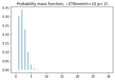
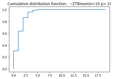
Let \(P(z)\) denote the probability generating function of a binomial distribution.
\(p_{0}\) is \(p_{0}=P[z=0]\).
The probability generating function of a Zero-Truncated binomial is defined in equation (20).
Example code on the usage of the ZTBinom class:
from gemact import distributions
import numpy as np

n=10
p=.2
dist=distributions.ZTBinom(n=n, p=p)
seq=np.arange(0,30,.001)
nsim=int(1e+05)

# Compute the mean via pmf
mean=np.sum(dist.pmf(seq)*seq)
variance=np.sum(dist.pmf(seq)*(seq-mean)**2)

print('Mean',mean)
print('Variance',variance)
#compare with simulations
print('Simulated mean',np.mean(dist.rvs(nsim)))
print('Simulated variance',np.var(dist.rvs(nsim)))
Then, use matplotlib library to show the pmf and the cdf of a ZTBinom:
import matplotlib.pyplot as plt

#pmf
plt.vlines(x=seq, ymin=0, ymax=dist.pmf(seq))
plt.title('Probability mass function, ~ZTBinom(n=10 p=.2)')


#cdf
plt.step(np.arange(0,20),dist.cdf(np.arange(0,20)),'-', where='pre')
plt.title('Cumulative distribution function,  ~ZTBinom(n=10 p=.2)')
ZMBinom#
Parametrization#
Let \(P(z)\) denote the probability generating function of a binomial distribution.
\(p_{0}\) is \(p_{0}=P[z=0]\).
The probability generating function of a Zero-Truncated binomial is defined in equation (21)
Example code on the usage of the ZMBinom class:
from gemact import distributions
import numpy as np

n=10
p=.2
p0m=.05
dist=distributions.ZMBinom(n=n,p=p,p0m=p0m)
seq=np.arange(0,100,.001)
nsim=int(1e+05)

# Compute the mean via pmf
mean=np.sum(dist.pmf(seq)*seq)
variance=np.sum(dist.pmf(seq)*(seq-mean)**2)

print('Mean',mean)
print('Variance',variance)
#compare with simulations
print('Simulated mean',np.mean(dist.rvs(nsim)))
print('Simulated variance',np.var(dist.rvs(nsim)))
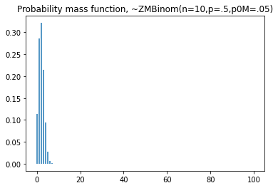
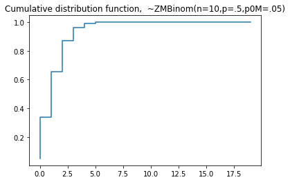
Then, use matplotlib library to show the pmf and the cdf of a ZMPoisson:
import matplotlib.pyplot as plt

#pmf
plt.vlines(x=seq, ymin=0, ymax=dist.pmf(seq))
plt.title('Probability mass function, ~ZMBinom(n=10,p=.5,p0m=.05)')

#cdf
plt.step(np.arange(0,20),dist.cdf(np.arange(0,20)),'-', where='pre')
plt.title('Cumulative distribution function,  ~ZMBinom(n=10,p=.5,p0m=.05)')
ZTGeom#
Parametrization#
Let \(P(z)\) denote the probability generating function of a geometric distribution.
\(p_{0}\) is \(p_{0}=P[z=0]\).
The probability generating function of a Zero-Truncated geometric is defined in equation (22).
Example code on the usage of the ZTGeom class:
from gemact import distributions
import numpy as np

p=.2
dist=distributions.ZTGeom(p=p)
seq=np.arange(0,100,.001)
nsim=int(1e+05)

# Compute the mean via pmf
mean=np.sum(dist.pmf(seq)*seq)
variance=np.sum(dist.pmf(seq)*(seq-mean)**2)

print('Mean',mean)
print('Variance',variance)
#compare with simulations
print('Simulated mean',np.mean(dist.rvs(nsim)))
print('Simulated variance',np.var(dist.rvs(nsim)))
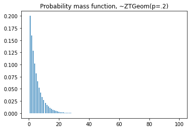
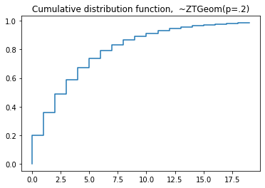
Then, use matplotlib library to show the pmf and the cdf of a ZTGeom:
import matplotlib.pyplot as plt

#pmf
plt.vlines(x=seq, ymin=0, ymax=dist.pmf(seq))
plt.title('Probability mass function, ~ZTGeom(p=.2)')
#cdf
plt.step(np.arange(0,20),dist.cdf(np.arange(0,20)),'-', where='pre')
plt.title('Cumulative distribution function,  ~ZTGeom(p=.2)')
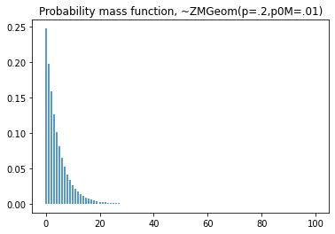
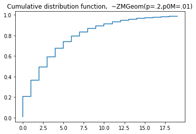
ZMGeom#
Parametrization#
Let \(P(z)\) denote the probability generating function of a geometric distribution.
\(p_{0}\) is \(p_{0}=P[z=0]\).
The probability generating function of a Zero-Modified geometric is defined in equation (23).
Example code on the usage of the ZMGeom class:
from gemact import distributions
import numpy as np

p=.2
p0m=.01
dist=distributions.ZMGeom(p=p,p0m=p0m)
seq=np.arange(0,100,.001)
nsim=int(1e+05)

# Compute the mean via pmf
mean=np.sum(dist.pmf(seq)*seq)
variance=np.sum(dist.pmf(seq)*(seq-mean)**2)

print('Mean',mean)
print('Variance',variance)
#compare with simulations
print('Simulated mean',np.mean(dist.rvs(nsim)))
print('Simulated variance',np.var(dist.rvs(nsim)))
Then, use matplotlib library to show the pmf and the cdf of a ZMGeom:
import matplotlib.pyplot as plt

#pmf
plt.vlines(x=seq, ymin=0, ymax=dist.pmf(seq))
plt.title('Probability mass function, ~ZMGeom(p=.2,p0m=.01)')

#cdf
plt.step(np.arange(0,20),dist.cdf(np.arange(0,20)),'-', where='pre')
plt.title('Cumulative distribution function,  ~ZMGeom(p=.2,p0m=.01)')
ZTNegBinom#
Parametrization#
Let \(P(z)\) denote the probability generating function of a negative binomial distribution.
\(p_{0}\) is \(p_{0}=P[z=0]\).
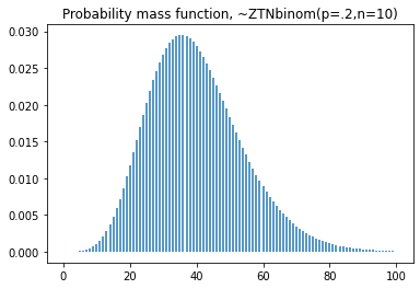
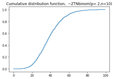
The probability generating function of a Zero-Truncated negative binomial is defined in equation (24).
Example code on the usage of the ZTNegBinom class:
from gemact import distributions
import numpy as np

p=.2
n=10
dist=distributions.ZTNegBinom(p=p,n=n)
seq=np.arange(0,100,.001)
nsim=int(1e+05)

# Compute the mean via pmf
mean=np.sum(dist.pmf(seq)*seq)
variance=np.sum(dist.pmf(seq)*(seq-mean)**2)

print('Mean',mean)
print('Variance',variance)
#compare with simulations
print('Simulated mean',np.mean(dist.rvs(nsim)))
print('Simulated variance',np.var(dist.rvs(nsim)))
Then, use matplotlib library to show the pmf and the cdf of a ZTNbinom:
import matplotlib.pyplot as plt

#pmf
plt.vlines(x=seq, ymin=0, ymax=dist.pmf(seq))
plt.title('Probability mass function, ~ZTNegBinom(p=.2,n=10)')

#cdf
plt.step(np.arange(0,100),dist.cdf(np.arange(0,100)),'-', where='pre')
plt.title('Cumulative distribution function,  ~ZTNegBinom(p=.2,n=10)')
ZMNegBinom#
Parametrization#
Let \(P(z)\) denote the probability generating function of a negative binomial distribution.
\(p_{0}\) is \(p_{0}=P[z=0]\).
The probability generating function of a Zero-Modified negative binomial is defined in equation (25).
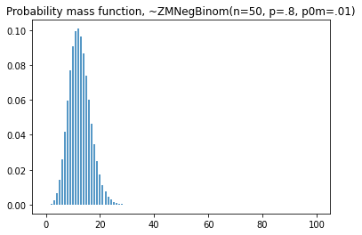
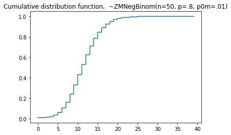
Example code on the usage of the ZMNegBinom class:
from gemact import distributions
import numpy as np

p=.2
n=100
p0M=.2
dist=distributions.ZMNegBinom(n=50,
                            p=.8,
                            p0m=.01)
seq=np.arange(0,100,.001)
nsim=int(1e+05)

# Compute the mean via pmf
mean=np.sum(dist.pmf(seq)*seq)
variance=np.sum(dist.pmf(seq)*(seq-mean)**2)

print('Mean',mean)
print('Variance',variance)
#compare with simulations
print('Simulated mean',np.mean(dist.rvs(nsim)))
print('Simulated variance',np.var(dist.rvs(nsim)))
Then, use matplotlib library to show the pmf and the cdf of a ZMNbinom:
import matplotlib.pyplot as plt

#pmf
plt.vlines(x=seq, ymin=0, ymax=dist.pmf(seq))
plt.title('Probability mass function, ~ZMNegBinom(p=.2,n=10)')

#cdf
plt.step(np.arange(0,100),dist.cdf(np.arange(0,100)),'-', where='pre')
plt.title('Cumulative distribution function,  ~ZMNegBinom(p=.2,n=10)')
ZMLogser#
Parametrization#
Let \(P(z)\) denote the probability generating function of a logarithmic distribution.
\(p_{0}\) is \(p_{0}=P[z=0]\).
The probability generating function of a Zero-Modified logarithmic is defined in equation (26).
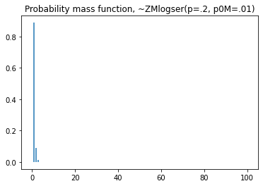
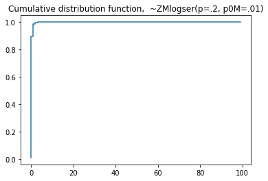
Example code on the usage of the ZMLogser class:
from gemact import distributions
import numpy as np

p=.2
p0m=.01
dist=distributions.ZMlogser(p=p,p0m=p0m)
seq=np.arange(0,100,.001)
nsim=int(1e+05)

# Compute the mean via pmf
mean=np.sum(dist.pmf(seq)*seq)
variance=np.sum(dist.pmf(seq)*(seq-mean)**2)

print('Mean',mean)
print('Variance',variance)
#compare with simulations
print('Simulated mean',np.mean(dist.rvs(nsim)))
print('Simulated variance',np.var(dist.rvs(nsim)))
Then, use matplotlib library to show the pmf and the cdf of a ZMlogser:
import matplotlib.pyplot as plt

#pmf
plt.vlines(x=seq, ymin=0, ymax=dist.pmf(seq))
plt.title('Probability mass function, ~ZMlogser(p=.2, p0m=.01)')
#cdf
plt.step(np.arange(0,10),dist.cdf(np.arange(0,10)),'-', where='pre')
plt.title('Cumulative distribution function,  ~ZMlogser(p=.2, p0m=.01)')
Gamma#
Parametrization#
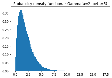
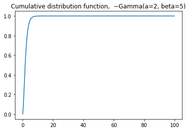
For a better explanation refer to the SciPy Gamma distribution documentation, see Virtanen et al. [VGO+20].
Given \(f(x, a)=\frac{x^{a-1} e^{-x}}{\Gamma(a)}\) and \(x \geq 0, a>0\). \(\Gamma(a)\) refers to the gamma function.
Example code on the usage of the Gamma class:
from gemact import distributions
import numpy as np

a=2
b=5
dist=distributions.Gamma(a=a,
                         beta=b)
seq=np.arange(0,100,.1)
nsim=int(1e+05)

print('Theorical mean',dist.mean())
print('Theorical variance',dist.var())
#compare with simulations
print('Simulated mean',np.mean(dist.rvs(nsim)))
print('Simulated variance',np.var(dist.rvs(nsim)))
Then, use matplotlib library to show the pmf and the cdf of a Gamma:
import matplotlib.pyplot as plt

#pmf
plt.hist(dist.rvs(nsim),
         bins=100,
         density=True)
plt.title('Probability density function, ~Gamma(a=2, beta=5)')
#cdf
plt.plot(seq,dist.cdf(seq))
plt.title('Cumulative distribution function,  ~Gamma(a=2, beta=5)')
Exponential#
Parametrization#
Given \(\theta \geq 0\).
Example code on the usage of the Exponential class:
from gemact import distributions
import numpy as np

theta=.1
dist=distributions.Exponential(theta=theta)
seq=np.arange(0,200,.1)
nsim=int(1e+05)

print('Theorical mean',dist.mean())
print('Theorical variance',dist.var())
#compare with simulations
print('Simulated mean',np.mean(dist.rvs(nsim)))
print('Simulated variance',np.var(dist.rvs(nsim)))
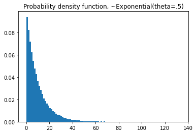
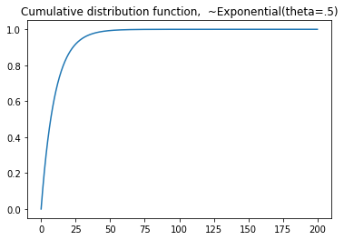
Then, use matplotlib library to show the pmf and the cdf of an Exponential:
import matplotlib.pyplot as plt

#pmf
plt.hist(dist.rvs(nsim),
         bins=100,
         density=True)
plt.title('Probability density function, ~Gamma(a=2, beta=5)')
#cdf
plt.plot(seq,dist.cdf(seq))
plt.title('Cumulative distribution function,  ~Gamma(a=2, beta=5)')
InvGauss#
Parametrization#
For a better explanation refer to the SciPy InvGauss distribution documentation, see Virtanen et al. [VGO+20].
InvGamma#
Parametrization#
For a better explanation refer to the SciPy Inverse Gamma distribution documentation, see Virtanen et al. [VGO+20]. Virtanen et al. [VGO+20].
Given \(x>=0, a>0 `. :math:\)Gamma(a)` refers to the gamma function.
GenPareto#
Parametrization#
For a better explanation refer to the SciPy documentation, see Virtanen et al. [VGO+20].
Given \(x \geq 0\) if \(c \geq 0\). \(0 \leq x \leq-1 / c if c<0\).
Example code on the usage of the GenPareto class:
from gemact import distributions
import numpy as np

c=.4
loc=0
scale=0.25

dist=distributions.Genpareto(c=c,
                            loc=loc,
                            scale=scale)

seq=np.arange(0,100,.1)
nsim=int(1e+05)

print('Theorical mean',dist.mean())
print('Theorical variance',dist.var())
#compare with simulations
print('Simulated mean',np.mean(dist.rvs(nsim)))
print('Simulated variance',np.var(dist.rvs(nsim)))
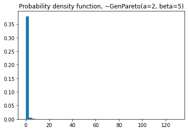
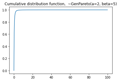
Then, use matplotlib library to show the pmf and the cdf of a GenPareto:
import matplotlib.pyplot as plt

#pmf
plt.hist(dist.rvs(nsim),
         bins=50,
         density=True)
plt.title('Probability density function, ~GenPareto(a=2, beta=5)')

#cdf
plt.plot(seq,dist.cdf(seq))
plt.title('Cumulative distribution function,  ~GenPareto(a=2, beta=5)')
Pareto2#
Parametrization#
Given \(x>m,-\infty<m<\infty, 1/s>0 p>0\).
Example code on the usage of the Pareto2 class:
from gemact import distributions
import numpy as np

s=2
dist=distributions.Pareto2(s=.9)

seq=np.arange(0,100,.1)
nsim=int(1e+08)
Pareto1#
Lognormal#
Parametrization#
For a better explanation refer to the SciPy Lognormal distribution documentation, see Virtanen et al. [VGO+20].
Given \(x>0, s>0\).
Example code on the usage of the Lognormal class:
from gemact import distributions
import numpy as np

s=2
dist=distributions.Lognorm(s=s)

seq=np.arange(0,100,.1)
nsim=int(1e+08)

print('Theorical mean',dist.mean())
print('Theorical variance',dist.var())
#compare with simulations
print('Simulated mean',np.mean(dist.rvs(nsim)))
print('Simulated variance',np.var(dist.rvs(nsim)))
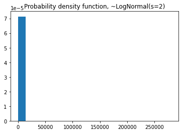
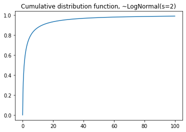
Then, use matplotlib library to show the pmf and the cdf of a LogNorm:
import matplotlib.pyplot as plt
#pmf
plt.hist(dist.rvs(nsim),
         bins=20,
         density=True)
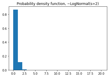
plt.title('Probability density function, ~LogNormal(s=2)')
#cdf
plt.plot(seq,dist.cdf(seq))
plt.title('Cumulative distribution function, ~LogNormal(s=2)')
Burr12#
Parametrization#
For a better explanation refer to the Scipy Burr12 distribution documentation , see Virtanen et al. [VGO+20].
Given \(x>=0 and c, d>0\).
Example code on the usage of the Burr12 class:
from gemact import distributions
import numpy as np

c=2
d=3
dist=distributions.Burr12(c=c,
                          d=d)

seq=np.arange(0,100,.1)
nsim=int(1e+05)

print('Theorical mean',dist.mean())
print('Theorical variance',dist.var())
#compare with simulations
print('Simulated mean',np.mean(dist.rvs(nsim)))
print('Simulated variance',np.var(dist.rvs(nsim)))
Then, use matplotlib library to show the pmf and the cdf of a Burr12:
import matplotlib.pyplot as plt

#pmf
plt.hist(dist.rvs(nsim),
         bins=100,
         density=True)
plt.title('Probability density function, ~Burr12(c=c,d=d)')

#cdf
plt.plot(seq,dist.cdf(seq))
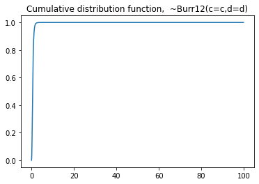
plt.title('Cumulative distribution function,  ~Burr12(c=c,d=d)')
Paralogistic#
Parametrization#
Given \(x>=0 and a >0\).
Example code on the usage of the Paralogistic class:
from gemact import distributions
import numpy as np

a=2

dist=distributions.Paralogistic(a=a)

seq=np.arange(0,100,.1)
nsim=int(1e+05)

print('Theorical mean',dist.mean())
print('Theorical variance',dist.var())
#compare with simulations
print('Simulated mean',np.mean(dist.rvs(nsim)))
print('Simulated variance',np.var(dist.rvs(nsim)))
Then, use matplotlib library to show the pmf and the cdf of a Burr12:
import matplotlib.pyplot as plt

#pmf
plt.hist(dist.rvs(nsim),
         bins=100,
         density=True)
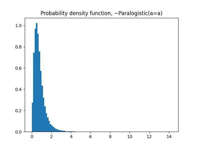
plt.title('Probability density function, ~Paralogistic(a=a)')

#cdf
plt.plot(seq,dist.cdf(seq))
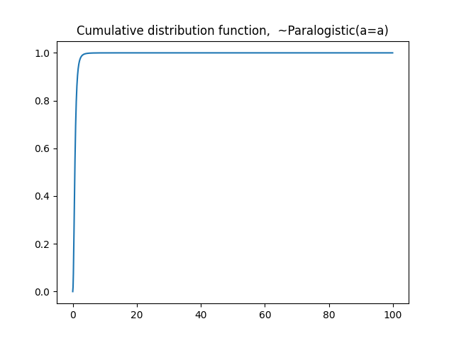
plt.title('Cumulative distribution function,  ~Paralogistic(a=a)')
Dagum#
Parametrization#
For a better explanation refer to the SciPy Dagum distribution documentation ,see Virtanen et al. [VGO+20].
Given \(x>0\) , \(k,s>0\).
Example code on the usage of the Dagum class:
from gemact import distributions
import numpy as np

d=2
s=4.2
dist=distributions.Dagum(d=d,
                         s=s)

seq=np.arange(0,3,.001)
nsim=int(1e+05)

print('Theorical mean',dist.mean())
print('Theorical variance',dist.var())
#compare with simulations
print('Simulated mean',np.mean(dist.rvs(nsim)))
print('Simulated variance',np.var(dist.rvs(nsim)))
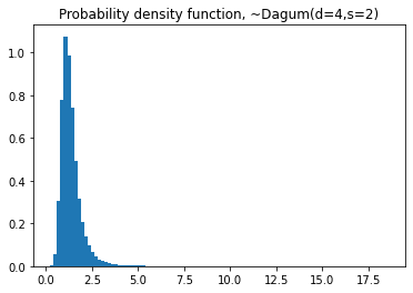
Then, use matplotlib library to show the pmf and the cdf of a Dagum:
import matplotlib.pyplot as plt

#pmf
plt.hist(dist.rvs(nsim),
         bins=100,
         density=True)
plt.title('Probability density function, ~Dagum(d=4,s=2)')

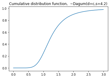
#cdf
plt.plot(seq,dist.cdf(seq))
plt.title('Cumulative distribution function,  ~Dagum(d=c,s=4.2)')
Inverse Paralogistic#
Parametrization#
Given \(x>0\) , \(b>0\).
Example code on the usage of the InvParalogistic class:
from gemact import distributions
import numpy as np

b=2
dist=distributions.InvParalogistic(b=b)

seq=np.arange(0,3,.001)
nsim=int(1e+05)

print('Theorical mean',dist.mean())
print('Theorical variance',dist.var())
#compare with simulations
print('Simulated mean',np.mean(dist.rvs(nsim)))
print('Simulated variance',np.var(dist.rvs(nsim)))
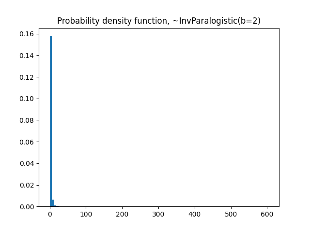
Then, use matplotlib library to show the pmf and the cdf of a Dagum:
import matplotlib.pyplot as plt

#pmf
plt.hist(dist.rvs(nsim),
         bins=100,
         density=True)
plt.title('Probability density function, ~InvParalogistic(b=2)')

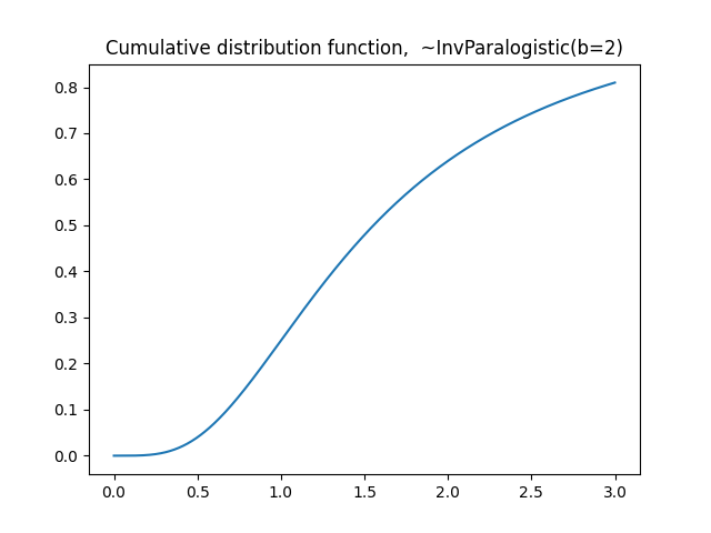
#cdf
plt.plot(seq,dist.cdf(seq))
plt.title('Cumulative distribution function,  ~InvParalogistic(b=2)')
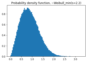
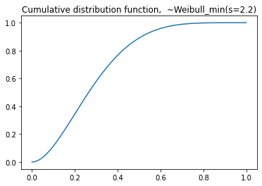
Weibull#
Parametrization#
For a better explanation refer to the SciPy Weibull distribution documentation , see Virtanen et al. [VGO+20].
Given \(x>0\) , \(c>0\).
Example code on the usage of the Weibull class:
from gemact import distributions
import numpy as np

c=2.2
dist=distributions.Weibull_min(c=c)

seq=np.arange(0,3,.001)
nsim=int(1e+05)

print('Theorical mean',dist.mean())
print('Theorical variance',dist.var())
#compare with simulations
print('Simulated mean',np.mean(dist.rvs(nsim)))
print('Simulated variance',np.var(dist.rvs(nsim)))
Then, use matplotlib library to show the pmf and the cdf of a Weibull_min:
import matplotlib.pyplot as plt

#pmf
plt.hist(dist.rvs(nsim),
         bins=100,
         density=True)
plt.title('Probability density function, ~Weibull_min(s=2.2)')

#cdf
plt.plot(seq,dist.cdf(seq))
plt.title('Cumulative distribution function,  ~Invweibull(c=7.2)')
InvWeibull#
Parametrization#
For a better explanation refer to the`Scipy Inverse Weibull distribution documentation <https://docs.scipy.org/doc/scipy/reference/generated/scipy.stats.invweibull.html>`_ Virtanen et al. [VGO+20] .
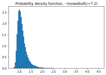
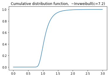
Given \(x>0\) , \(c>0\).
Example code on the usage of the InvWeibull class:
from gemact import distributions
import numpy as np

c=7.2
dist=distributions.Invweibull(c=c)

seq=np.arange(0,3,.001)
nsim=int(1e+05)

print('Theorical mean',dist.mean())
print('Theorical variance',dist.var())
#compare with simulations
print('Simulated mean',np.mean(dist.rvs(nsim)))
print('Simulated variance',np.var(dist.rvs(nsim)))
Then, use matplotlib library to show the pmf and the cdf of a Invweibull:
import matplotlib.pyplot as plt

#pmf
plt.hist(dist.rvs(nsim),
         bins=100,
         density=True)
plt.title('Probability density function, ~Invweibull(c=7.2)')
#cdf
plt.plot(seq,dist.cdf(seq))
plt.title('Cumulative distribution function,  ~Invweibull(c=7.2)')
Beta#
Parametrization#
For a better explanation refer to the SciPy Beta distribution documentation, Virtanen et al. [VGO+20] .
Given \(0<=x<=1, a>0, b>0\) , \(\Gamma\) is the gamma function.
Example code on the usage of the Beta class:
from gemact import distributions
import numpy as np

a=2
b=5
dist=distributions.Beta(a=a,
                        b=b)

seq=np.arange(0,1,.001)
nsim=int(1e+05)

print('Theorical mean',dist.mean())
print('Theorical variance',dist.var())
#compare with simulations
print('Simulated mean',np.mean(dist.rvs(nsim)))
print('Simulated variance',np.var(dist.rvs(nsim)))
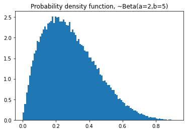
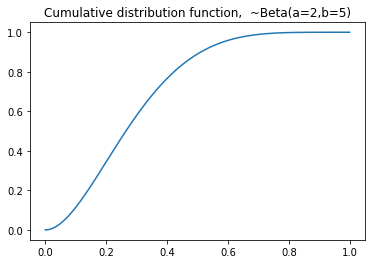
Then, use matplotlib library to show the pmf and the cdf of a Beta:
import matplotlib.pyplot as plt

#pmf
plt.hist(dist.rvs(nsim),
         bins=100,
         density=True)
plt.title('Probability density function, ~Beta(a=2,b=5)')
#cdf
plt.plot(seq,dist.cdf(seq))
plt.title('Cumulative distribution function,  ~Beta(a=2,b=5)')
Loggamma#
Parametrization#
where \(x>0, \alpha>0, \lambda >0\) and \(\Gamma(\alpha)\) is the Gamma function.
GenBeta#
Parametrization#
Given \(0<=x<=scale, shape_1>0, shape_2>0\) , \(\Gamma\) is the gamma function.
Example code on the usage of the GenBeta class:
from gemact import distributions
import numpy as np

shape1=1
shape2=2
shape3=3
scale=4

dist=GenBeta(shape1=shape1,
             shape2=shape2,
             shape3=shape3,
             scale=scale)

seq=np.arange(0,1,.001)
nsim=int(1e+05)

print('Theorical mean',dist.mean())
print('Theorical variance',dist.var())
#compare with simulations
print('Simulated mean',np.mean(dist.rvs(nsim)))
print('Simulated variance',np.var(dist.rvs(nsim)))
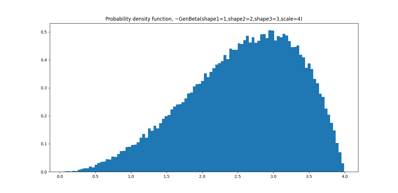
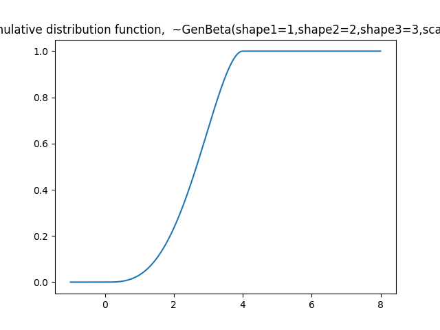
Then, use matplotlib library to show the pmf and the cdf of a GenBeta:
import matplotlib.pyplot as plt

#pmf
plt.hist(dist.rvs(nsim),
         bins=100,
         density=True)
plt.title('Probability density function, ~GenBeta(shape1=1,shape2=2,shape3=3,scale=4)')
#cdf
plt.plot(np.arange(-1,8,.001),dist.cdf(np.arange(-1,8,.001)))
plt.title('Cumulative distribution function,  ~GenBeta(shape1=1,shape2=2,shape3=3,scale=4)')
Multinomial#
Parametrization#
The multinomial probability mass function is given by
where \(\sum_{i=1}^k x_i = n\), \(x_i \in \mathbb{N}_0\), \(p_i \ge 0\) and \(\sum_{i=1}^k p_i = 1\).
Example code on the usage of the Multinomial class:
from gemact import distributions

dist = distributions.Multinomial(n=10, p=[0.2, 0.3, 0.5])
x = [2, 3, 5]

print('PMF at x:', dist.pmf(x))
print('Mean vector:', dist.mean())
print('Random variates:\n', dist.rvs(size=3, random_state=42))
Dirichlet_Multinomial#
Parametrization#
Let \(\alpha_0 = \sum_{i=1}^k \alpha_i\). The Dirichlet-multinomial mass function is
where \(x_i \in \mathbb{N}_0\), \(\sum_{i=1}^k x_i = n\) and \(\alpha_i > 0\) for all \(i\).
Example code on the usage of the Dirichlet_Multinomial class:
from gemact import distributions

dist = distributions.Dirichlet_Multinomial(n=12, alpha=[2.0, 3.0, 4.0], seed=7)
x = [4, 5, 3]

print('PMF at x:', dist.pmf(x))
print('Mean vector:', dist.mean())
print('Random variates:\n', dist.rvs(size=2, random_state=21))
NegMultinom#
Parametrization#
Let \(p_0 = 1 - \sum_{i=1}^k p_i\). The negative multinomial mass function is
where \(x_0 > 0\), \(x_i \in \mathbb{N}_0\), \(p_i \ge 0\) and \(\sum_{i=1}^k p_i < 1\).
Example code on the usage of the NegMultinom class:
from gemact import distributions
import numpy as np

dist = distributions.NegMultinom(x0=5, p=[0.2, 0.3])
x = np.array([3, 4])

print('PMF at x:', dist.pmf(x))
print('Mean vector:', dist.mean())
print('Covariance matrix:\n', dist.cov())
MultivariateBinomial#
Parametrization#
The multivariate binomial vector \(\mathbf{X} = (X_1,\ldots,X_k)\) models the number of successes in \(n\) common Bernoulli trials with success probabilities \(p_i = \Pr(B_i = 1)\) and pairwise joint success probabilities \(p_{ij} = \Pr(B_i = 1, B_j = 1)\) for each coordinate. The marginal distributions are binomial with
while the dependence structure is governed by \(p_{ij}\). The first two moments are
Example code on the usage of the MultivariateBinomial class:
from gemact import distributions
import numpy as np

p_joint = np.array([[0.3, 0.12, 0.10],
                    [0.12, 0.4, 0.08],
                    [0.10, 0.08, 0.35]])

dist = distributions.MultivariateBinomial(n=20, p_joint=p_joint)
x = np.array([5, 6, 4])

print('PMF at x:', dist.pmf(x))
print('Mean vector:', dist.mean())
print('Covariance matrix:\n', dist.cov())
MultivariatePoisson#
Parametrization#
Let \(\mathbf{X} = (X_1,\ldots,X_k)\) be a multivariate Poisson vector with marginal means \(\mu_i\) and pairwise joint intensities \(\lambda_{ij}\). Each component can be represented as
where \(Y_i \sim \mathrm{Poisson}\left(\mu_i - \sum_{j \ne i} \lambda_{ij}\right)\) and \(Y_{ij} = Y_{ji} \sim \mathrm{Poisson}(\lambda_{ij})\) are independent. Consequently,
Example code on the usage of the MultivariatePoisson class:
from gemact import distributions
import numpy as np

mu = np.array([2.0, 3.0, 1.5])
mu_joint = np.array([[0.0, 0.4, 0.2],
                     [0.4, 0.0, 0.3],
                     [0.2, 0.3, 0.0]])

dist = distributions.MultivariatePoisson(mu=mu, mu_joint=mu_joint)
x = np.array([1, 2, 0])

print('PMF at x:', dist.pmf(x))
print('Mean vector:', dist.mean())
print('Covariance matrix:\n', dist.cov())
print('Random variates:\n', dist.rvs(size=5, random_state=123))
The copulas module#
Guide to copulas
ClaytonCopula#
Parametrization#
Clayton copula cumulative density function:
Given \(u_{k} \in[0,1], k=1, \ldots, d\) , \(\delta > 0\) .
Example code on the usage of the ClaytonCopula class:
from gemact import copulas

clayton_c=copulas.ClaytonCopula(par=1.4,
                                dim=2)
clayton_c.rvs(size=100,
              random_state= 42)
FrankCopula#
Parametrization#
Frank copula cumulative density function:
Given \(u_{k} \in[0,1], k=1, \ldots, d\) , \(\delta >= 0\) .
Example code on the usage of the FrankCopula class:
from gemact import copulas
frank_c=copulas.FrankCopula(par=1.4,
                            dim=2)
frank_c.rvs(size=100,
              random_state= 42)
GumbelCopula#
Parametrization#
Gumbel copula cumulative density function:
Given \(u_{k} \in[0,1], k=1, \ldots, d\) , \(\delta >= 1\) .
Example code on the usage of the GumbelCopula class:
from gemact import copulas

gumbel_c=copulas.GumbelCopula(par=1.4,
                              dim=2)
gumbel_c.rvs(size=100,
              random_state= 42)
GaussCopula#
Parametrization#
Gauss copula cumulative density function is based on the scipy function multivariate_normal. For a better explanation refer to the SciPy Multivariate Normal documentation, Virtanen et al. [VGO+20] .
Example code on the usage of the GaussCopula class:
from gemact import copulas

corr_mx=np.array([[1,.4],[.4,1]])

gauss_c=copulas.GaussCopula(corr=corr_mx)
gauss_c.rvs(size=100,
              random_state= 42)
TCopula#
Parametrization#
T copula cumulative density function:
Given \(u_{k} \in[0,1], k=1, \ldots, d\). \(t_{v}^{-1}\) is the inverse student’s t function and \(\boldsymbol{t}_{v, C}\) is the cumulative distribution function of the multivariate student’s t distribution with a given mean and correlation matrix C. Degrees of freedom \(v>0\) .
Example code on the usage of the TCopula class:
from gemact import copulas

corr_mx=np.array([[1,.4],[.4,1]])

t_c=copulas.TCopula(corr=corr_mx,
                    df=5)
t_c.rvs(size=100,
        random_state= 42)
Independence Copula#
Parametrization#
Independence Copula.
Given \(u_{k} \in[0,1], k=1, \ldots, d\).
Example code on the usage of the IndependentCopula class:
from gemact import copulas

i_c = copulas.IndependentCopula(dim=2)
i_c.rvs(1,random_state=42)
Fréchet–Hoeffding Lower Bound#
Parametrization#
The Fréchet–Hoeffding Lower Bound Copula.
Given \(u_{k} \in[0,1], k=1, 2\).
Example code on the usage of the FHLowerCopula class:
from gemact import copulas

fhl_c = copulas.FHLowerCopula
fhl_c.rvs(10,
        random_state=42)
Fréchet–Hoeffding Upper Bound#
Parametrization#
The Fréchet–Hoeffding Upper Bound Copula.
Given \(u_{k} \in[0,1], k=1, 2\).
Example code on the usage of the FHUpperCopula class:
from gemact import copulas

fhu_c = copulas.FHUpperCopula
fhu_c.rvs(10,
        random_state=42)
References#
Philipp Arbenz, Paul Embrechts, and Giovanni Puccetti. The aep algorithm for the fast computation of the distribution of the sum of dependent random variables. Bernoulli, 17:562–591, 2011.
P. Embrechts and M. Frei. Panjer recursion versus fft for compound distributions. Mathematical Methods of Operations Research, 2008.
Wayne H. Fisher, Jeffrey T. Lange, and John Balcarek. Loss reserve testing: a report year approach. 1999.
Alessandro Ricotta and Gian Paolo Clemente. An extension of collective risk model for stochastic claim reserving. 2016.
Nino Savelli and Gian Paolo Clemente. Lezioni di matematica attuariale delle assicurazioni danni. EDUCatt-Ente per il diritto allo studio universitario dell'Università Cattolica, 2014. ISBN 9788867807048. URL: http://hdl.handle.net/10807/67154.
B. Sundt. On excess of loss reinsurance with reinstatements. Insurance: Mathematics and Economics, 1991.
Pauli Virtanen, Ralf Gommers, Travis E. Oliphant, Matt Haberland, Tyler Reddy, David Cournapeau, Evgeni Burovski, Pearu Peterson, Warren Weckesser, Jonathan Bright, Stéfan J. van der Walt, Matthew Brett, Joshua Wilson, K. Jarrod Millman, Nikolay Mayorov, Andrew R. J. Nelson, Eric Jones, Robert Kern, Eric Larson, C J Carey, İlhan Polat, Yu Feng, Eric W. Moore, Jake VanderPlas, Denis Laxalde, Josef Perktold, Robert Cimrman, Ian Henriksen, E. A. Quintero, Charles R. Harris, Anne M. Archibald, Antônio H. Ribeiro, Fabian Pedregosa, Paul van Mulbregt, and SciPy 1.0 Contributors. SciPy 1.0: Fundamental Algorithms for Scientific Computing in Python. Nature Methods, 17:261–272, 2020. doi:10.1038/s41592-019-0686-2.
